Optimization Techniques

Double Buffering

Double buffering is a term used to describe a device with two buffers. The usage of multiple buffers increases the overall throughput of a device and helps prevents bottlenecks. For example, with graphics, double buffering can show one image or frame while a separate frame is being buffered to be shown next. This method makes animations and games look more realistic than the same done in a single buffer mode.

Cache Blocking

An important class of algorithmic changes involves blocking data structures to fit in cache. By organizing data memory accesses, one can load the cache with a small subset of a much larger data set. The idea is then to work on this block of data in cache. By using/reusing this data in cache we reduce the need to go to memory (reduce memory bandwidth pressure. The key idea behind blocking is to exploit the inherent data reuse available in the application by ensuring that data remains in cache across multiple uses.

In terms of code change, blocking typically involves a combination of loop splitting and interchange. In most application codes,

Original Source:

1
2
3
4
5

for (body1 = 0; body1 < NBODIES; body1 ++) {
   for (body2=0; body2 < NBODIES; body2++) {
     OUT[body1] += compute(body1, body2);
   }
}

In this example, data (body2) is streamed from memory. Assuming NBODIES is large, we would have no reuse in cache. This application is memory bandwidth bound. The application will run at the speed of memory to CPU speeds, less than optimal.

Modified Source (with 1-D blocking):

1
2
3
4
5
6
7

for (body2 = 0; body2 < NBODIES; body2 += BLOCK) {
   for (body1=0; body1 < NBODIES; body1 ++) {
      for (body22=0; body22 < BLOCK; body22 ++) {
         OUT[body1] += compute(body1, body2 + body22);
      }
   }
}

In this modified code, data (body22) is kept and reused in cache, resulting in better performance. If BLOCK is chosen such that this set of values fits in cache, memory traffic is brought down by a factor of BLOCK.

Example:

 1
 2
 3
 4
 5
 6
 7
 8
 9
10
11
12
13
14
15
16
17
18
19
20
21
22
23
24
25
26
27
28
29
30
31
32
33
34
35
36

#include <iostream>
#include <ctime>

using namespace std;
int main() {
  int size = 4000000;
  int b_size = 1000;
  double* A= new double [size];
  double* B = new double [b_size];
  for (int i = 0; i < size; i++)
    A[i] = 1;
  clock_t start, end;
  start = clock();
  for (int i = 0; i < b_size; i++) {
    for (int j = 0; j < size; j++) {
      B[i] += A[j];
    }
  }
  end = clock();
  cout << "normal cost time: " << end - start << endl;

  start = clock();
  int block = 4000;
  for (int b = 0; b < size / block; b++) {
    for (int i = 0; i < b_size; i++) {
      for (int j = 0; j < block; j++) {
        B[i] += A[j];
      }
    }
  }
  end = clock();
  cout << "cache blocking cost time: " << end - start << endl;
  delete [] A;
  delete [] B;
  return 0;
}

normal cost time: 10503367

cache blocking cost time: 9575784

Keep Memory

In order to avoid unnecessary reallocation and release, we can keep some reused parameters (such as modle parameters) in the core memory.

Memory Coalescing and cache utilization

Main memory gets loaded via cache line chunks - usually 64 or 128 bytes - through a hierarchy of caches: from DRAM to L3 to L2 and L1 and finally to the CPU registers.Modern cache sizes have increased significantly, and we can have around 35MB of space in L3 cache shared with all the processors. Reading from L3 cache is approximately 3x faster than from DRAM.

In order to utilizing this feature, we should removing data memory fragmentation. The following are some examples:

• While facing sparse input vectors or matrix, we can create one long contiguous vector that consecutively stores non-zero indices and values. To keep track of variable numbers of non-zeros, we keep another vector of offsets.

• In neural networks, the neuron weights in the same layer can be located contiguously in the main memory increasing cache efficiency.

Hyper-threading

Hyper-Threading allows the processor to virtually double its number of cores and execute twice as many threads simultaneously, jumping back and forth between threads to execute instructions for one whenever the other is stalled.

• If the program need randomly access the memory, threads do get stalled due to cache miss. At that point, hyper-threading will be favorable because another thread can utilize the wait time to process a different data instance.

Vectorization

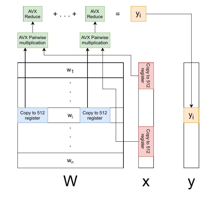
Matrix-vector multiplication, matrix in store in row-major.

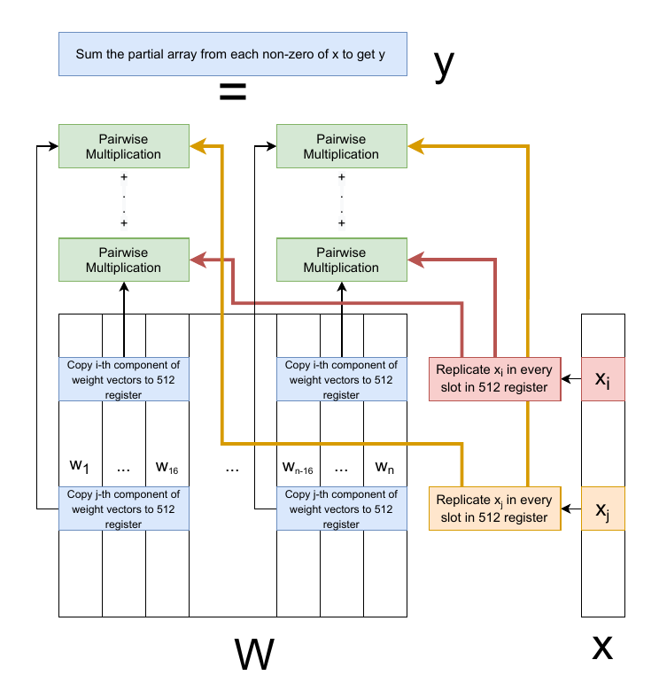
Matrix-vector multiplication, matrix in store in column-major.

Memory Reuse

To reduce the memory allocate and destroy.

Branch Prediction

 1
 2
 3
 4
 5
 6
 7
 8
 9
10
11
12
13
14
15
16
17
18
19
20
21
22
23
24
25
26
27
28
29
30
31
32

#include <vector>
#include <chrono>
#include <iostream>
#include <algorithm>

using namespace std;

int main(){
    const unsigned arraySize = 32768;
    int data[arraySize];
    //生成0-255范围的随机数并存入数组data
    for(unsigned c = 0;c<arraySize;++c){
        data[c] = std::rand() % 256;
    }
  	//对数组进行排序
    std::sort(data,data + arraySize);

    auto start = chrono::system_clock::now();
    long long sum = 0;
    for(unsigned i = 0;i<100000;++i){
        for(unsigned c = 0; c < arraySize; ++c){
            if(data[c] >= 128){
                sum += data[c];
            }
        }
    }
    auto end = chrono::system_clock::now();
    auto duration = chrono::duration_cast<chrono::microseconds>(end-start);
    double elapsed  = double(duration.count()) * chrono::microseconds::period::num / chrono::microseconds::period::den;
    std::cout << "Time cost：" << elapsed <<" s" << std::endl;
    std::cout << "sum =" << sum << std::endl;
}

After sort the array the time cost is: 5 s

Without sort the time cost is: 15 s

The reason is than the CPU using branch predition strategy, after sort could increase the branch prediction accuracy.

We could replace the conditional branch by some hack skill, eg..

1
2
3
4
5
6
7

if (a >= 128) {
    sum += a;
}
// replace by follow

int t = (a - 128) >> 31;
sum += ~t & a;

NUMA-aware

Reference

1. Introduction to Instruction Scheduling
2. Memory Optimizations
3. Accelerating SLIDE Deep Learning on Modern CPUs: Vectorization, Quantizations, Memory Optimizations and More
4. SLIDE : IN DEFENSE OF SMART ALGORITHMS OVER HARDWARE ACCELERATION FOR LARGE -SCALE DEEP LEARNING SYSTEMS
5. NUMA-Caffe: NUMA-Aware Deep Learning Neural Networks